← Curriculum index·L0 · Project Overview · xBD + ATC-20 L1 · Vision Transformers L2 · Focal Loss, Dice Loss & Class Weights L3 · Siamese Neural Networks L4 · Encoder · ResNet-50 L5 · Decoder · U-Net L6 · Ablation Study L7 · Hyper-parameters

Lecture L3

Siamese Neural Networks

Architecture, variants and theory — from Bell Labs signature verification (1993) to modern xBD pre/post damage assessment.

Shared encoderDifference blockSkip connectionsAttention gatesDeep supervisionContrastive / TripletVanishing gradient proof

In plain English — read this first

What is a Siamese network? Two identical copies of the same neural network running side by side. Both copies share the exact same weights — that is what "Siamese" means here (like identical twins). You feed one copy the "before" image and the other copy the "after" image, then compare what each one saw.

Why two copies? For disaster damage we don't really care what a building looks like in isolation — we care about what changed between the pre-event and post-event photo. The cleanest way to ask "what changed?" is to run both photos through the same eyes (same weights), then subtract the answers. That subtraction is the difference block: D = | F_post − F_pre |.

The four ideas you need before reading on:

Shared weights — both branches use the same parameters θ. If one branch learns "this is a roof", the other branch automatically learns the same. Without sharing, the two branches would drift apart and the comparison would be meaningless.
Feature map — what comes out of an encoder. Not a picture, but a stack of numerical maps where each map highlights a different pattern (edges, textures, roofs, debris…).
Difference block — the absolute difference of the two feature maps. Large values mean "this patch changed a lot" — exactly the change-detection signal we want.
Skip + attention — the difference is fed sideways into a U-Net decoder via skip connections, while attention gates suppress noisy areas (clouds, shadows) so the model focuses on real structural change.

Analogy: a Siamese network is like asking two identical inspectors to walk the same street before and after a storm, then computing the difference in their notes. Because the inspectors are clones, any disagreement is evidence of real change — not personal style.

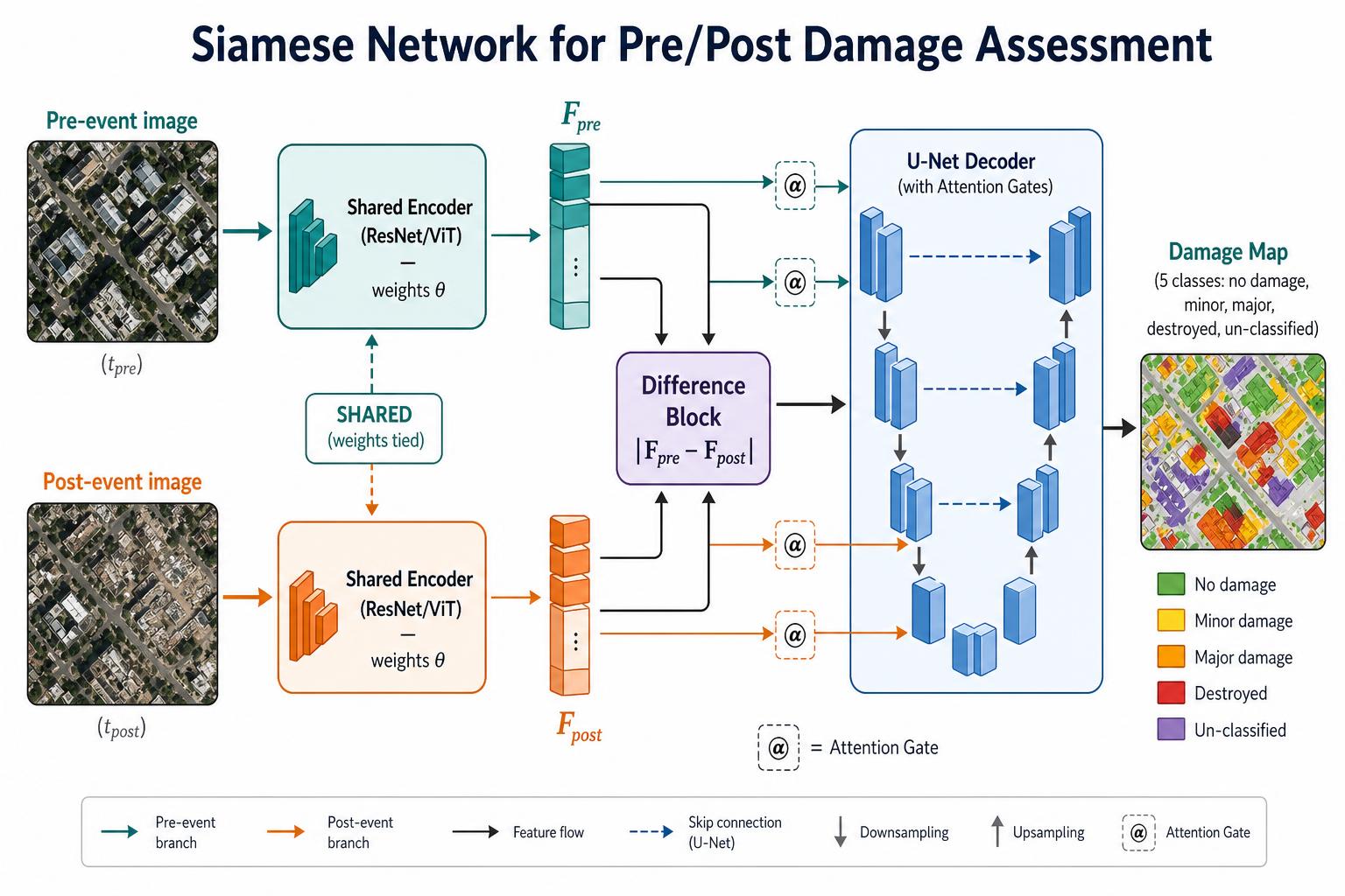
Siamese network for pre/post damage assessment: pre- and post-event satellite images each pass through a shared encoder with tied weights θ, producing F_pre and F_post. A difference block |F_pre − F_post| feeds a U-Net decoder with attention gates and skip connections, outputting a 5-class damage map. — **Figure 1.** Siamese twin encoders (shared weights θ) compare pre- and post-event imagery via a difference block; a U-Net decoder with attention gates produces the per-pixel damage map.

Figure walkthrough — read the diagram block by block

① Pre-event image (t_pre) — a satellite photo of a neighbourhood before the disaster. Top (teal) branch of the network.
② Post-event image (t_post) — the same geographic location after the disaster. Bottom (orange) branch. Both images must be co-registered (aligned pixel-for-pixel).
③ Shared Encoder (ResNet / ViT) — weights θ — a CNN or ViT backbone that turns each image into a compact feature map. The dashed "SHARED (weights tied)" arrow means both branches are literally the same network, just run twice. Updating θ updates both branches at once → pre and post are described in the same feature space, which is what makes subtraction meaningful.
④ F_pre and F_post — the two feature tensors that come out of the encoder. Each one summarises "what is in this image" at a coarse spatial resolution (e.g. 32×32×512).
⑤ Difference Block |F_pre − F_post| — element-wise absolute difference. Pixels that did not change cancel out (→ 0); pixels that changed (collapsed roofs, debris) light up. This is the change signal the decoder will turn into a damage map.
⑥ Skip connections (dashed arrows into the decoder) — U-Net style. They route fine-grained features from each encoder stage directly to the matching decoder stage, restoring the spatial detail that pooling discarded → sharp building outlines instead of blobs.
⑦ Attention Gates (the @ boxes) — small learned gates on each skip connection that ask "which skip pixels are actually relevant for this output region?" and suppress the rest. Cuts false positives on background (roads, trees).
⑧ U-Net Decoder — progressively upsamples the difference features back to full image resolution, fusing them with the gated skip features at every stage.
⑨ Damage Map (5 classes) — the final per-pixel prediction, colour-coded: green = no damage, yellow = minor, orange = major, red = destroyed, purple = un-classified. Argmax over the 5 channels gives each pixel its label.
Arrow legend — solid teal/orange = the two image branches, solid black = feature flow, dashed blue = U-Net skip connection, @ = attention gate. The down-arrow inside the decoder is downsampling, the up-arrow is upsampling.

What is a Siamese Network?

Origins, intuition, and the core idea.

A Siamese network is a neural architecture containing two (or more) identical sub-networks that share the same weights. Each branch processes a different input; their outputs are compared to produce a similarity score or difference map.

Bromley et al. (1993) — Bell Labs, signature verification. The original "Siamese" twin network.
Koch et al. (2015) — one-shot image classification via contrastive loss.
Modern uses — face verification (FaceID-style), satellite change detection (xBD), medical image comparison, self-supervised learning (SimSiam, BYOL).

Why "Siamese"?

Two branches share weights — like Siamese twins sharing a body. Updating one updates the other. They are literally the same network, run twice.

Four key properties

① Shared weights · ② Symmetric · ③ Comparison output · ④ Half the parameters of two separate nets.

Core Architecture for xBD Damage Assessment

Pre-event (t₁)  ──▶ [Shared Encoder θ] ──▶ F_pre  ┐
                                                  ├─▶ Difference Block |F_pre − F_post| ─▶ Decoder ─▶ Damage map (5 classes)
Post-event (t₂) ──▶ [Shared Encoder θ] ──▶ F_post ┘                                                    │
                                                                                                      ▼
                                                                                          Combined Loss = Focal + Dice
                                                                                                      │
                                                              ◀──── Backprop (updates ONE shared encoder θ) ────

Pre/post inputs — 512×512×3 satellite images of the same geographic location at two times.
Shared encoder — ResNet-50/101 or ViT, parameters θ₁ = θ₂. Output: feature maps [C × H/8 × W/8].
Difference block — |F_pre − F_post| (or learned fusion). Highlights what changed.
Decoder — upsamples H/8 → H/4 → H/2 → H with skip connections from encoder stages.
Output — [5 × H × W] tensor; argmax gives per-pixel damage class.

Inside the Shared Encoder

Conv → BN → ReLU → pool, four times.

Input 512×512×3
  → Conv Block 1  → 256×256×64   (stride 2, 64 filters)
  → Conv Block 2  → 128×128×128
  → Conv Block 3  →  64×64×256
  → Conv Block 4  →  32×32×512   ← Feature map for comparison

Conv 3×3

Extracts local edges, textures, shapes.

BatchNorm

x̂ = (x−μ)/(σ+ε); y = γx̂+β. Keeps activations healthy → stable gradients.

ReLU

f(x)=max(0,x). Non-linearity that does not saturate for positive inputs (unlike sigmoid).

Decoder — Skip Connections & Attention Gates

U-Net-style skip connections route encoder features directly to the matching decoder stage, restoring spatial detail that pooling discarded.

Decoder stage k:
  u_k     = Upsample( d_{k-1} )                  # coarse decoder features
  skip_k  = Encoder feature at same resolution
  d_k     = Conv( Concat[ u_k, AttentionGate(skip_k, u_k) ] )

# Attention gate (Oktay et al., 2018)
α = σ( ψ( ReLU( W_x · x + W_g · g ) ) )           # gate ∈ [0,1] per pixel
gated_skip = α ⊙ x

The attention gate lets the decoder ask "which encoder pixels are relevant here?" and suppresses the rest — sharper boundaries, fewer false positives on background.

Loss Functions for Siamese Training

Loss	Formula	When to use
Contrastive	L = y·D² + (1−y)·max(0, m−D)²	Pairwise similarity (face verify, signature)
Triplet	L = max(0, D(a,p) − D(a,n) + m)	Anchor/positive/negative — face recognition
Focal	−α(1−pₜ)^γ log(pₜ)	Imbalanced segmentation (damage)
Dice	1 − 2\|A∩B\| / (\|A\|+\|B\|)	Region overlap — boundary quality
Focal + Dice	L_F + L_D	DAHiTrA / xBD damage assessment ✓

Siamese Variants

Variant	Key idea	When to use
Classic Siamese	Two identical branches, shared θ	Same modality, same domain (xBD)
Pseudo-Siamese	Same architecture, separate θ	Slight domain shift (e.g. different sensors)
Asymmetric	Different architectures per branch	Cross-modality (RGB vs SAR, optical vs infrared)
Triplet	Three branches (anchor/pos/neg), shared θ	Metric learning, face recognition
Self-supervised (SimSiam / BYOL / DINO)	Two augmented views of one image	Label-scarce pre-training

Vanishing Gradient — Cause & Cure

Why deep Siamese stacks need help, and how skip connections + deep supervision fix it.

Plain deep network — gradient at the input

\frac{\partial \mathcal{L}}{\partial x_0} \;=\; \frac{\partial \mathcal{L}}{\partial x_L}\;\prod_{\ell=0}^{L-1}\frac{\partial f_{\ell}}{\partial x_{\ell}}

where

$x_{\ell}$ — activation entering layer \ell
$f_{\ell}$ — the transformation applied by layer \ell
$L$ — total depth

The gradient at the input is a product of L Jacobians. If most of them have magnitude less than 1, the product shrinks geometrically — by the time it reaches $x_0$ there is almost nothing left to learn from. This is the classic vanishing-gradient problem.

Residual block — vanishing problem cured

\begin{aligned} x_{\ell+1} &= f_{\ell}(x_{\ell}) + x_{\ell} \\[6pt] \frac{\partial x_{\ell+1}}{\partial x_{\ell}} &= \frac{\partial f_{\ell}}{\partial x_{\ell}} + I \end{aligned}

where

$+\,x_{\ell}$ — skip connection — adds the input back to the layer's output
$I$ — identity matrix that the skip contributes to the Jacobian

Each factor in the product is now at least the identity. Even if a layer's learned mapping has tiny gradient, the $+\,I$ guarantees a healthy floor — gradient survives all the way back to the early Siamese encoder layers.

Deep supervision goes further by attaching auxiliary Focal+Dice losses at intermediate decoder stages, so early encoder layers get strong gradient signal directly — not only through a long chain.

PyTorch — Minimal Siamese Skeleton

python
1import torch, torch.nn as nn
2
3class SharedEncoder(nn.Module):
4    def __init__(self):
5        super().__init__()
6        # e.g. ResNet-50 backbone, output [B, 512, H/8, W/8]
7        self.backbone = build_resnet50_encoder()
8
9    def forward(self, x):
10        return self.backbone(x)
11
12class SiameseDamageNet(nn.Module):
13    def __init__(self, num_classes=5):
14        super().__init__()
15        self.encoder = SharedEncoder()     # ONE encoder, used twice
16        self.decoder = UNetDecoder(in_channels=512, out_channels=num_classes)
17
18    def forward(self, pre, post):
19        f_pre  = self.encoder(pre)         # shared weights θ
20        f_post = self.encoder(post)        # same θ — literally same nn.Module
21        diff   = torch.abs(f_pre - f_post) # change signal
22        return self.decoder(diff)          # [B, 5, H, W] damage logits
23
24# Training (with Focal + Dice from L2)
25model = SiameseDamageNet().cuda()
26optim = torch.optim.AdamW(model.parameters(), lr=1e-4, weight_decay=1e-4)
27
28for pre, post, mask in loader:
29    logits = model(pre.cuda(), post.cuda())
30    loss   = focal_fn(logits, mask.cuda().long()) + dice_fn(logits, one_hot(mask))
31    optim.zero_grad(); loss.backward(); optim.step()

Which variant for which task?

Task	Recommended variant	Loss
xBD building damage (pre/post)	Classic Siamese + UNet decoder	Focal + Dice + deep supervision
Signature / face verification	Classic Siamese, embedding head	Contrastive or Triplet
Optical vs SAR change detection	Asymmetric Siamese	Focal + Dice
Self-supervised pre-training	SimSiam / BYOL / DINO	Cosine similarity (no negatives)
One-shot classification	Classic Siamese	Contrastive

Key takeaway

Siamese = one encoder run twice + a comparison. Shared weights guarantee that pre and post are described in the same feature space — so subtraction is meaningful. Combined with Focal+Dice and deep supervision, it is the canonical architecture for modern disaster damage assessment.

Triplet Loss — pull positives close, push negatives away

The standard metric-learning loss for Siamese / verification networks.

A triplet is three samples: an anchor $a$ (e.g. a building in the pre-event image), a positive $p$ (the same building in the post-event image — should look similar in feature space), and a negative $n$ (a different building, or a destroyed one — should look far away). Each sample is pushed through the same encoder $f_\theta$ to an embedding vector.

\mathcal{L}_{\text{triplet}}(a,p,n) \;=\; \max\!\bigl(\,0,\ \ \|f(a)-f(p)\|_2^{\,2} \;-\; \|f(a)-f(n)\|_2^{\,2} \;+\; m\,\bigr)

Margin $m$ — the gap (typically 0.2–1.0) that the negative must exceed the positive by. Without it, the trivial solution $f(x)=0$ would minimise the loss.
Hinge / max(0,·) — once the negative is already $m$ further than the positive, the triplet contributes zero gradient. Training focuses only on still-violating triplets.
Gradient intuition — for a violating triplet, the encoder is pulled so $f(a)\to f(p)$ and pushed so $f(a)\to$ away from $f(n)$ , simultaneously.

Triplet mining — which triples do you actually train on?

Strategy	Definition	Use when
Random	Sample (a,p,n) uniformly at random.	Quick sanity tests; converges slowly.
Easy	n is already far away → loss ≈ 0.	Avoid — provides no gradient.
Semi-hard	‖f(a)−f(n)‖ > ‖f(a)−f(p)‖ but still inside the margin.	FaceNet-style training — best stability.
Hard	n closer to a than p is.	Strong signal but can collapse without warm-up.

python
1import torch, torch.nn as nn, torch.nn.functional as F
2
3class TripletLoss(nn.Module):
4    def __init__(self, margin=0.3):
5        super().__init__()
6        self.margin = margin
7    def forward(self, anchor, positive, negative):
8        # L2-normalise so distances live on the unit sphere (recommended)
9        a = F.normalize(anchor,  dim=1)
10        p = F.normalize(positive, dim=1)
11        n = F.normalize(negative, dim=1)
12        d_pos = (a - p).pow(2).sum(dim=1)   # ‖a - p‖²
13        d_neg = (a - n).pow(2).sum(dim=1)   # ‖a - n‖²
14        return F.relu(d_pos - d_neg + self.margin).mean()
15
16# Use with a triplet sampler that emits (anchor, positive, negative) batches
17# from the xBD index — same building (pre vs post) = positive,
18# different building = negative.

Triplet vs. Contrastive

Contrastive loss needs pairs + a binary label (same / different). Triplet loss needs three samples but no explicit label — the structure of (anchor, positive, negative) carries the signal. Triplet typically gives sharper embeddings because every update encodes a relative constraint (n must be further than p), not an absolute one.

Cosine Distance — angle, not magnitude

The default metric for embedding spaces.

Cosine similarity measures the angle between two vectors, ignoring how long they are:

\cos(u, v) \;=\; \frac{u \cdot v}{\|u\|\,\|v\|} \;\in\; [-1, 1] \qquad d_{\cos}(u,v) \;=\; 1 - \cos(u, v) \;\in\; [0, 2]

Relation to dot product

If both vectors are L2-normalised (i.e. $\|u\|=\|v\|=1$ ), then cosine similarity collapses to the plain dot product: $\cos(u,v)=u\cdot v$ . In code that's one line:

python
1u = F.normalize(u, dim=1)
2v = F.normalize(v, dim=1)
3sim = (u * v).sum(dim=1)   # ∈ [-1, 1]
4dist = 1.0 - sim           # ∈ [0, 2]

Relation to L2 on the unit sphere

For unit vectors, the squared Euclidean distance is exactly twice the cosine distance:

\|u-v\|_2^2 \;=\; 2\,(1 - u\!\cdot\! v) \;=\; 2\,d_{\cos}(u,v)

So a triplet loss with L2-normalised embeddings is mathematically a triplet loss in cosine space. Most modern face/verification systems do exactly this.

When to use	Cosine distance	Euclidean (L2) distance
Embedding magnitude is meaningless (text, image features)	Yes — angle is all that matters	No — long vectors dominate
Pixel-space comparison	No — direction ignores intensity	Yes — captures absolute change
Mixed-norm vectors (different L2 lengths)	Yes — magnitude-invariant	No — bias toward larger vectors
High-dimensional embeddings (CLIP, ViT, face nets)	Yes — the de-facto standard	Use only after L2-normalisation

Practical recipe

Train with triplet loss after L2-normalising the encoder outputs. At inference, declare two buildings 'the same' if

d_{\cos}(f(a), f(b)) < \tau

(tune

\tau

on the validation set, typically 0.2–0.4 for sharp embeddings).

Acronyms & jargon — quick reference

Siamese: — two identical branches sharing the same weights, run on two inputs.
θ (theta): — the network's learnable weights. "Shared θ" means both branches use the same numbers.
F_pre, F_post: — feature maps (stacks of pattern maps) from the pre- and post-event images.
Difference block: — |F_pre − F_post|: bright where pixels changed, zero where they didn't.
U-Net: — encoder-decoder shape with skip connections; standard for image-to-image tasks.
Skip connection: — wire from an early encoder layer straight to the decoder, restoring fine detail.
Attention gate: — learned 0–1 mask on a skip that says "use this region, ignore that one".
ResNet: — CNN family with residual (skip) connections; the "50" = 50 layers deep.
ViT: — Vision Transformer: encodes images as a sequence of patches with self-attention.
BN (BatchNorm): — normalises activations per mini-batch so training stays stable.
ReLU: — activation max(0,x): keep positives, zero negatives.
Jacobian: — matrix of partial derivatives of a layer's output w.r.t. its input.
Vanishing gradient: — gradient shrinks toward 0 as it travels back through many layers → early layers stop learning.
Contrastive / Triplet: — Siamese losses that pull "same" pairs close and push "different" pairs apart in feature space.